From a SAXS curve to lipid-nanoparticle structure
A SAXS measurement of lipid nanoparticles (LNPs) gives you a one-dimensional curve. This page walks through how that curve becomes a structural readout of the particle population, in concepts rather than code. General scientific background is assumed; no SAXS or machine-learning expertise required.
The code, tutorials, and full technical reference are in the GitHub repository.
What does a SAXS experiment give us?
Small-angle X-ray scattering (SAXS) is a measurement performed on a liquid sample of nanoparticles in solution, without freezing or staining them. X-rays are scattered by electron-density variations inside the particles. The scattered radiation forms a two-dimensional ring pattern on the detector; averaging azimuthally around the centre collapses this pattern into a single one-dimensional curve, scattered intensity as a function of the wavevector q (a quantity related to the angle of scattering).
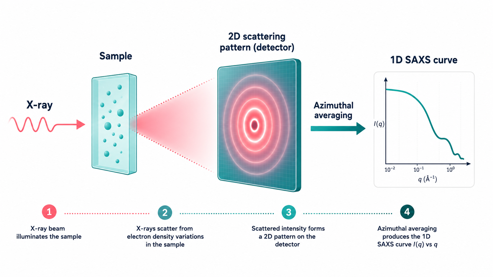
That curve carries information about the particles in the sample. Specifically, it encodes the spatial distribution of electron density inside the particles, averaged over the whole population and over all particle orientations. Bigger particles scatter differently from smaller ones. Particles with a shell scatter differently from particles without one. Particles with rough interiors scatter differently from particles with uniform interiors.
There is one fundamental catch. The curve is one-dimensional. The structure is three-dimensional. Recovering 3D structure from a 1D curve is an underdetermined problem: more than one structure can be consistent with the same curve.
For uniform spherical particles, the model is analytical
The simplest case is a sample of identical, uniformly dense spherical particles. A closed-form formula, called the sphere form factor, predicts what their SAXS curve will look like given a single radius. To analyze the measurement, you adjust the radius until the predicted curve matches the data. Fast and clean.
Adding polydispersity stays in the analytical regime
Real samples never contain identical particles. Even the simplest gold-nanoparticle synthesis produces particles with a spread of sizes. This is called polydispersity, and it is a property of every real particle population.
Polydispersity is straightforward to add to the model: assume a distribution of radii (typically log-normal), and average the sphere form factor over that distribution. You now fit two numbers (the mean radius and its spread) instead of one. The polydispersity integral is fast, and the model stays analytical.
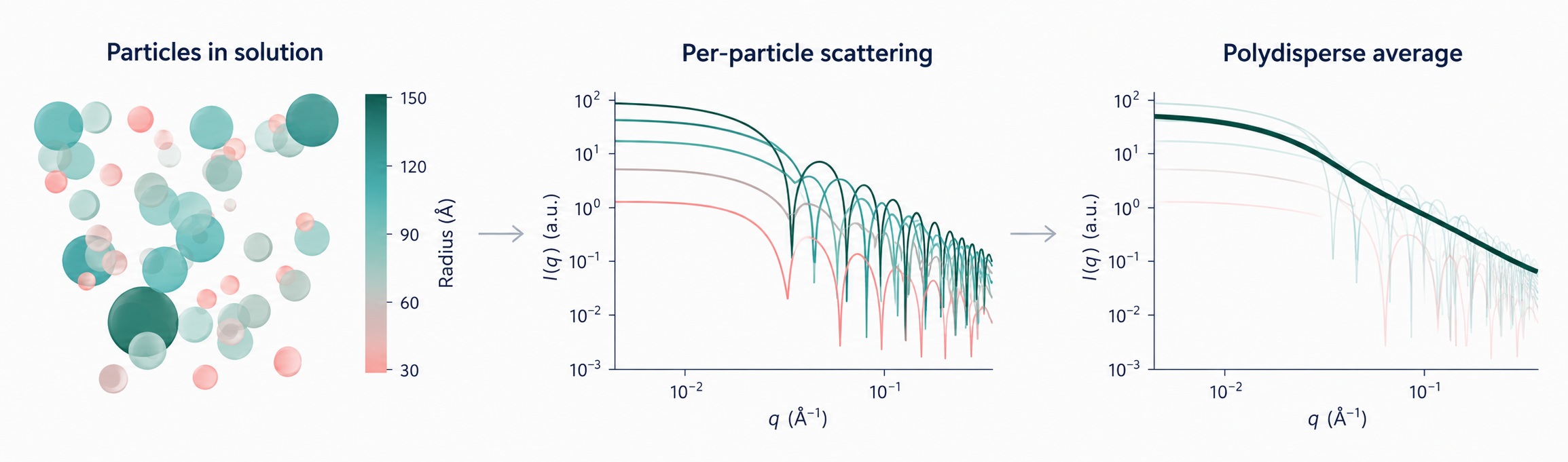
The smoothing is the key effect. Each individual radius produces a curve with sharp oscillations at distinct q values. The size-averaged curve inherits the shape of those individual curves at low q but loses the oscillations at high q: the minima from different radii fall at different q and fill each other in. What you measure on a real polydisperse sample is the smooth curve, and the spread of the curve (how quickly the high-q shape decays) carries information about the width of the radius distribution.
This is enough for many systems: gold nanoparticles, simple silica colloids, and any approximately spherical particle population that is roughly uniform inside. It is what the repository’s analytical path provides, with both a polydisperse sphere model and a polydisperse core-shell model. The gold tutorial walks through this on real experimental data.
Heterogeneous interiors break the analytical machinery
Lipid nanoparticles are different. Not because they are polydisperse (every real population is), but because what is inside them does not conform to any uniform density profile. They have a shell of lipids of some thickness and composition, and an interior of stochastically arranged lipids and cargo (often RNA). No simple closed-form formula captures this kind of structure.
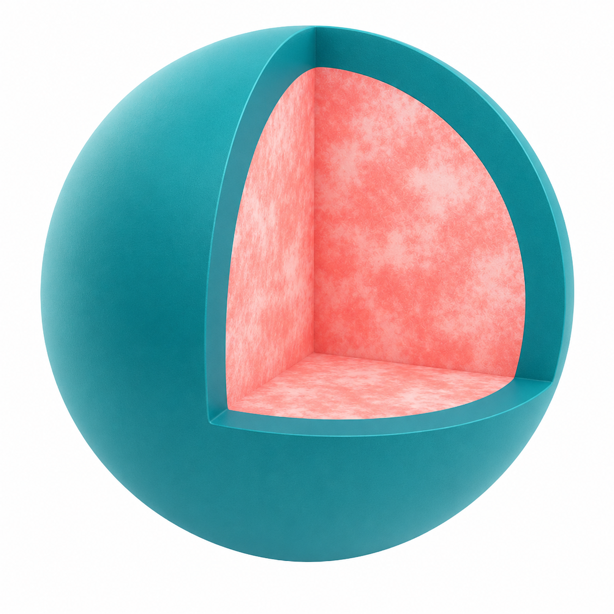
To analyze a SAXS measurement of these particles, you need a realistic numerical forward model: a model that actually constructs a particle (including a stochastic realization of its interior), computes its SAXS curve from electron-density principles, and averages over both the size distribution and the stochastic interior realizations.
This works in principle. In practice, it is far too slow. A single such forward computation takes seconds. To fit a measurement you need to perform thousands of these computations: each step of the optimizer asks for one, and you run the optimizer many times from different starting points to avoid local minima. Days of compute per fit become impractical.
The neural surrogate
This is the first thing the framework introduces. Note what the problem actually is. The slow numerical simulator is, on its own, already differentiable: implemented in JAX, it produces gradients of the predicted SAXS curve with respect to its physical inputs automatically. That is the same machinery that makes gradient-based fitting straightforward in the analytical case. Differentiability is not the bottleneck. Speed is. A single forward evaluation takes seconds, and we need thousands per fit.
We therefore train a neural network to mimic the simulator. The network learns, from thousands of simulator-generated examples, how the SAXS curve depends on the physical parameters that describe an LNP.
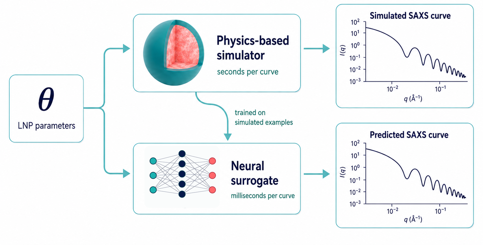
Once trained, the network is fast. Predictions take milliseconds rather than seconds. From the optimizer’s point of view it looks like the same forward model, just thousands of times quicker, and accurate enough that its predictions match the simulator well within the noise level of an experimental SAXS curve. With the surrogate in place, fitting an LNP SAXS curve becomes practical: hundreds of independent optimizations run in under a minute on a single GPU, a task that would otherwise take days.
What the paper covers
This overview stops at the forward problem and the surrogate. The framework also addresses a second issue, beyond speed. SAXS is a one-dimensional measurement of a three-dimensional structure, so many different parameter sets can produce nearly identical curves. A single best-fit number, taken on its own, is misleading. To make this visible, the framework retains an ensemble of near-optimal fits and examines which parameter directions the data constrains and which remain degenerate. The mathematical treatment, the identifiability analysis, and the synthetic and experimental validation are in the paper.
Further reading
- GitHub repository — code, tutorials, full technical reference.
- The paper (in preparation) for the mathematical treatment and the synthetic and experimental validation.